View on GitHub

Download Notebook

Plotting OpenFE results against experiment using Cinnabar v0.6.0

This notebook shows how one would go about creating a cinnabar style plot of OpenFE results against known experimental values. For more information on the cinnabar API and the available plot styles, see the tutorials.

Setup for Google Colab

If you are running this example in Google Colab, run the following cells to setup the environment. If you are running this notebook locally, skip down to Loading experimental data

# NBVAL_SKIP
# Only run this cell if on Google Colab
import os
if "COLAB_RELEASE_TAG" in os.environ:
    # fix for colab's torchvision causing issues
    !rm -r /usr/local/lib/python3.12/dist-packages/torchvision

    !pip install -q condacolab
    import condacolab
    condacolab.install_from_url("https://github.com/OpenFreeEnergy/openfe/releases/download/v1.7.0/OpenFEforge-1.7.0-Linux-x86_64.sh")

# NBVAL_SKIP
# Only run this cell if on google colab
import os
if "COLAB_RELEASE_TAG" in os.environ:
    import condacolab
    import locale
    locale.getpreferredencoding = lambda: "UTF-8"
    !mkdir inputs && cd inputs && openfe fetch rbfe-tutorial
    # quick fix for https://github.com/conda-incubator/condacolab/issues/75
    # if deprecation warnings persist, rerun this cell
    import warnings
    warnings.filterwarnings(action="ignore", message=r"datetime.datetime.utcnow")
    for _ in range(3):
      # Sometimes we have to re-run the check
      try:
        condacolab.check()
      except:
        pass
      else:
        break

Loading experimental data

First, we load the experimental data from a tab-separated values (TSV) file.

The format of the TSV file is as follows:

ligand  estimate (kcal/mol)     uncertainty (kcal/mol)

Important note: Please note that for now you must have an experimental entry for every ligand involved in your free energy network. In future versions of cinnabar this will no longer be needed.

# First we do a set of imports
%matplotlib inline
%config InlineBackend.figure_formats = ['svg']
import pandas as pd
from cinnabar import FEMap, plotting
from openff.units import unit

# read in the experimental data
experimental_data = pd.read_csv('experimental.tsv', sep="\t")
experimental_data

	ligand	estimate (kcal/mol)	uncertainty (kcal/mol)
0	lig_ejm_31	-9.57	0.18
1	lig_ejm_42	-9.81	0.18
2	lig_ejm_43	-8.29	0.18
3	lig_ejm_45	-9.59	0.18
4	lig_ejm_46	-11.35	0.17
5	lig_ejm_47	-9.73	0.18
6	lig_ejm_48	-9.03	0.18
7	lig_ejm_50	-9.01	0.18
8	lig_ejm_54	-10.57	0.18
9	lig_ejm_55	-9.24	0.18
10	lig_jmc_23	-11.74	0.18
11	lig_jmc_27	-11.31	0.17
12	lig_jmc_28	-11.01	0.18

Loading free energy results

Next we load in results from the TSV file created by running openfe gather --report ddg on a network of results from relative binding free energy calculations.

Please see the full RBFE gather command tutorial for more information.

# Read in calculated relative free energy results
calculated_data = pd.read_csv('final_results.tsv', sep="\t")
calculated_data

	ligand_i	ligand_j	DDG(i->j) (kcal/mol)	uncertainty (kcal/mol)
0	lig_ejm_31	lig_ejm_42	0.49	0.09
1	lig_ejm_31	lig_ejm_46	-0.73	0.10
2	lig_ejm_31	lig_ejm_47	0.00	0.20
3	lig_ejm_31	lig_ejm_48	0.50	0.20
4	lig_ejm_31	lig_ejm_50	0.94	0.07
5	lig_ejm_42	lig_ejm_43	1.20	0.10
6	lig_ejm_46	lig_jmc_23	-0.39	0.05
7	lig_ejm_46	lig_jmc_27	-0.60	0.10
8	lig_ejm_46	lig_jmc_28	-0.12	0.04

Creating a Cinnabar FEMap

Next we will use the cinnabar API to gather the experimental and calculated results into a single object which we can use to plot and analyse the network of results.

Note: The FEMap object requires estimates and uncertainties to have units attached to remove ambiguity in the data. When using OpenFE results, the units are always kcal/mol, so we can attach these units using the OpenFF Units API.

fe_map = FEMap()

# add the calculated data
for _, row in calculated_data.iterrows():
    fe_map.add_relative_calculation(
        # the ligand we are transforming from
        labelA=row['ligand_i'],
        # the ligand we are transforming to
        labelB=row['ligand_j'],
        # the computed relative free energy change for the transformation with units
        value=row["DDG(i->j) (kcal/mol)"] * unit.kilocalories_per_mole,
        # the uncertainty in the computed relative free energy change with units
        uncertainty=row["uncertainty (kcal/mol)"] * unit.kilocalories_per_mole,
        # the source of the data, can be any string but should be consistent across all data points from the same source
        source="openfe",
    )

# add the experimental data
for _, row in experimental_data.iterrows():
    fe_map.add_experimental_measurement(
        # the ligand for which we have an experimental measurement
        label=row['ligand'],
        # the experimental free energy for that ligand with units
        value=row['estimate (kcal/mol)'] * unit.kilocalories_per_mole,
        # the uncertainty in the experimental free energy with units
        uncertainty=row['uncertainty (kcal/mol)'] * unit.kilocalories_per_mole,
        # the source of the data, can be any string but should be consistent across all data points from the same source
        source="Experimental",
    )

Plotting the results using Cinnabar

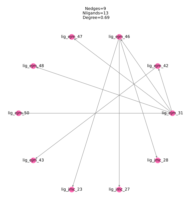
Once we’ve created the FEMap we can inspect the alchemical network:

fe_map.draw_graph()

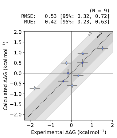
Plotting out the relative free energy results

Next we can go ahead and plot out the relative free energy results.

# note you can pass the filename argument to write things out to file
plotting.plot_DDGs(
    fe_map,
    source="openfe", # the name of the computational source to plot
    figsize=5
    )

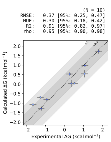
Plotting out the absolute free energy results

Finally let’s generate an estimate of the absolute binding free energy for each ligand using the MLE estimator and plot out the derived values:

# note you can pass the filename argument to write to file
fe_map.generate_absolute_values()  # Get MLE generated estimates of the absolute values
plotting.plot_DGs(
    fe_map,
    source="MLE", # the name of the computational source to plot
    figsize=5
    )

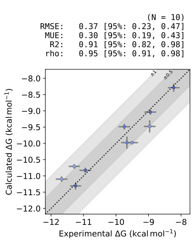
We can also shift our free energies by the average experimental value to have DGs on the same scale as experiment.

shift = experimental_data["estimate (kcal/mol)"].mean()  # shift the computed values by the mean of the experimental values to put them on a similar scale

plotting.plot_DGs(
    fe_map,
    source="MLE",
    figsize=5,
    shift=shift
)

Writing out the MLE derived absolute free energies

Finally, we can also extract the MLE derived absolute free energies along with the experimental results into a pandas DataFrame.

abs_df = fe_map.get_absolute_dataframe()
abs_df

	label	DG (kcal/mol)	uncertainty (kcal/mol)	source	computational
0	lig_ejm_31	-9.570	0.180000	Experimental	False
1	lig_ejm_42	-9.810	0.180000	Experimental	False
2	lig_ejm_43	-8.290	0.180000	Experimental	False
3	lig_ejm_45	-9.590	0.180000	Experimental	False
4	lig_ejm_46	-11.350	0.170000	Experimental	False
5	lig_ejm_47	-9.730	0.180000	Experimental	False
6	lig_ejm_48	-9.030	0.180000	Experimental	False
7	lig_ejm_50	-9.010	0.180000	Experimental	False
8	lig_ejm_54	-10.570	0.180000	Experimental	False
9	lig_ejm_55	-9.240	0.180000	Experimental	False
10	lig_jmc_23	-11.740	0.180000	Experimental	False
11	lig_jmc_27	-11.310	0.170000	Experimental	False
12	lig_jmc_28	-11.010	0.180000	Experimental	False
13	lig_ejm_31	0.041	0.054900	MLE	True
14	lig_ejm_42	0.531	0.088736	MLE	True
15	lig_ejm_43	1.731	0.125992	MLE	True
16	lig_ejm_46	-0.689	0.070810	MLE	True
17	lig_ejm_47	0.041	0.187120	MLE	True
18	lig_ejm_48	0.541	0.187120	MLE	True
19	lig_ejm_50	0.981	0.083271	MLE	True
20	lig_jmc_23	-1.079	0.083750	MLE	True
21	lig_jmc_27	-1.289	0.114079	MLE	True
22	lig_jmc_28	-0.809	0.079335	MLE	True

We can then extract the MLE derived values.

Note: you can obtain this directly from your results by calling ``openfe gather –report dg``

mle_df = abs_df[abs_df["source"] == "MLE"].reset_index(drop=True)
mle_df

	label	DG (kcal/mol)	uncertainty (kcal/mol)	source	computational
0	lig_ejm_31	0.041	0.054900	MLE	True
1	lig_ejm_42	0.531	0.088736	MLE	True
2	lig_ejm_43	1.731	0.125992	MLE	True
3	lig_ejm_46	-0.689	0.070810	MLE	True
4	lig_ejm_47	0.041	0.187120	MLE	True
5	lig_ejm_48	0.541	0.187120	MLE	True
6	lig_ejm_50	0.981	0.083271	MLE	True
7	lig_jmc_23	-1.079	0.083750	MLE	True
8	lig_jmc_27	-1.289	0.114079	MLE	True
9	lig_jmc_28	-0.809	0.079335	MLE	True